Tracking spheres in images (aka Let's Build a Half-Assed Playstation Move tracker!)

For fun, I decided to write basically a Playstation Move tracker. The idea is that you have some kind of glowing sphere with a known radius, take a picture of it with a camera, and infer where it is in 3D space. I bought these glowy balls since I don’t actually own a Playstation Move controller.

I ended up having some issues with my camera (possibly caused by running an internal windows build!) so I haven’t actually got around to the finishing off the full pipeline, but rather than let this sit around unifinished (possibly forever) I figured I’d at least write up what I have so far. Maybe there will be a part 2 in the future!

The setup

To have something to test with, I generated some images using D3D by rendering a sphere at a known position and radius with a known projection matrix. This allows me to at least get the basic math right and evaluate how well I can infer the original position from the image with synthetic noise/outliers. I use 8x MSAA and super-sampling to give me a bit of a gradient in the image (like you would get in a camera, where pixels aren’t unambiguously “on” or “off” the object).

Here’s an example of such an image. Knowing that e.g. the sphere in this image is exactly at the location (-0.5,0.75,-2) and has a radius of 0.2 we can use it to test our algorithm in a synthetic environment, before worrying too much about generating ground truth data with a real camera.

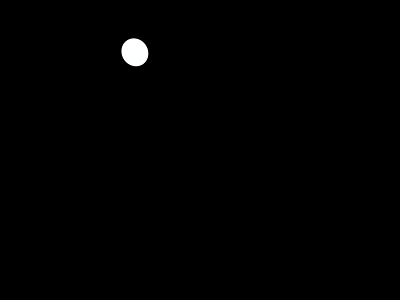
In reality, the image above would be the result of some image processing of a real image. For example, you may use a naive bayesian classifier based on image color pixels to produce a grayscale “sphere image mask” that simply tries to give a rough estimate of whether or not a given pixel is a sphere pixel or not. The rest of the post assumes we have such a sphere image mask (we will be robust to false positive outliers, though - it doesn’t have to be perfect). Here’s another input example where i just drew in some spurious shapes to simulate inputs where we have outliers that survive our sphere classification process (a lot more of them then I’d hope to see in real data).

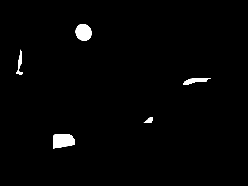
Once I get my camera working again I can use the built-in calibration data to give me a projection matrix (which we will use later), but if you’re following along at home with an standard webcam or something chances are it won’t come with calibration data and you’d need to run it through a calibration process like this one in order to find the camera matrix.

Finding the sphere edge pixels

In order to figure out where the sphere is, we’re just going to use the silhouette pixels. There are a few different ways of doing this. One way is to simply compute the gradient and spit out all the pixel locations whose gradient magnitude in the sphere image mask is larger than a threshold. This works, but unless you do something special, it loses sub-pixel information because the pixels aren’t actually binary black/white, they contain some information about where the edge of the sphere is in between pixels.

To take advantage of this extra grayscale information, we actually look at the current pixel and the one below and to the right, and if the pixel intensites go from being below some intensity threshold (we use 0.5 right now) to being above it, we interpolate to find the sub-pixel location where the cross-over point is, and output that as one of our edge points.

For example, if one pixel has an intensity of 0.25, and the next pixel to the right has an intensity of 0.65, we can expect that the true sphere edge to be slightly closer to the right pixel than the left.

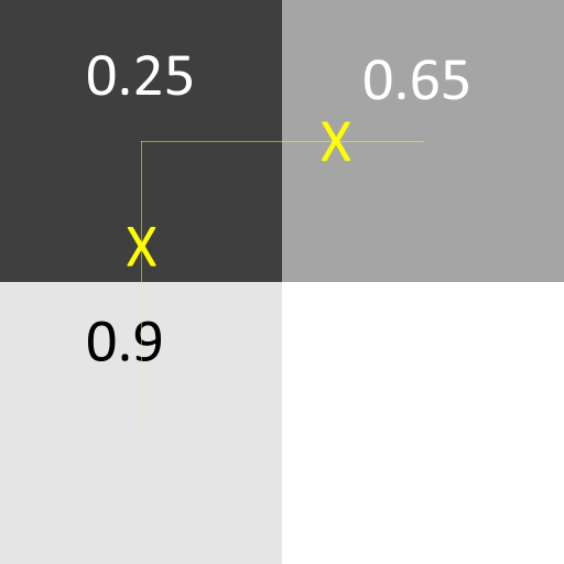
In the image above, you can see two such sub-pixel locations being determined using the differential intensity values.

Note, that in order for this to work you need to make sure your intensity values are linear and that 0.5 really does mean “intersecting the center of the pixel” (which in itself is an approximation at best). Depending on the camera this threshold value may need some tweaking, and maybe conversion from sRGB to linear.

There are more ways of getting sub-pixel information out of an image like this rather than using direct interpolation. For example, you can use an gradient magnitude threshold filter like I mentioned above, but later on when you optimize a position from all these edge pixels you could weight the cost function term from each pixel by the magnitude of the corresponding gradient. This means that sharp gradients get weighted higher whereas pixels that don’t straddle the edge quite so perfectly get a lower influence.

Another aproach is to weight the cost function term for each edge pixel by the reciprocal of the dot product of the gradient and the direction to the current candidate sphere center (plus some small epsilon to avoid divide by zero). This will tend to push the center towards a position such that most gradient vectors point toward it. This probably exploits the most information you can get out of the image since it takes into account both the orientation of the edge gradient and its magnitude, so in theory this might be the best approach.

I tried all three of these and in my admittedly limted test set there was no advantage to either, but I did get some benefit compared to using no sub-pixel information. So I decided to show the direct interpolation method described above because it’s a simple approach that makes the optimizer and cost function a bit less complicated (see later). It’s also a method I haven’t seen mentioned anywhere else so figured I’d throw that in the ring just in case I invented it or something.

 1 2 3 4 5 6 7 8 910111213141516171819202122232425262728293031323334353637

// Assume a pixel brighter than 50% gray is "inside" the circle
const float EDGE_SUBPIXEL_INTENSITY_THRESHOLD = 0.5f; 
std::vector<vec2> subPixelEdgePositions;
for (int y = 0; y + 1 < height; ++y)
{
	for (int x = 0; x + 1 < width; ++x)
	{			
		// Note: test data is linear for now, and all white. So just grab red channel. 
		// For real data, need to correct for sRGB and do some kind of RGB->Probability 
		// of being a sphere pixel classification first.
		float scale	= 1.0f / 255.0f;
		float topleft =	scale*imageBuf(x, y).x;
		float topright = scale*imageBuf(x+1, y).x;		
		float bottomleft = scale*imageBuf(x, y+1).x;
		
		// If neighbor pixels are on either side of the edge, linearly interpolate 
		// to find the subpixel position where the edge crosses and put that in our 
		// sub-pixel array. Note: we skip the right/bottom edges since they will be 
		// covered by another iteration of this loop.

		// top left -> top right
		if ((topleft < EDGE_SUBPIXEL_INTENSITY_THRESHOLD) ^ 
			(topright < EDGE_SUBPIXEL_INTENSITY_THRESHOLD))
		{
			float t = (EDGE_SUBPIXEL_INTENSITY_THRESHOLD-topleft) / (topright - topleft);
			subPixelEdgePositions.emplace_back(x + t,y);
		}

		// top left -> bottom left
		if ((topleft < EDGE_SUBPIXEL_INTENSITY_THRESHOLD) ^ 
			(bottomleft < EDGE_SUBPIXEL_INTENSITY_THRESHOLD))
		{
			float t = (EDGE_SUBPIXEL_INTENSITY_THRESHOLD-topleft) / (bottomleft - topleft);
			subPixelEdgePositions.emplace_back(x, y + t);
		}			
	}
}

Once we have the edge pixels we want, we can convert them to 3D rays in viewspace by simply multiplying by the inverse of the projection matrix. Like so:

12345678

std::vector<vec3> rayDirs;
rayDirs.reserve(subPixelEdgePositions.size());
for (vec2 pos : subPixelEdgePositions) {			
	vec2 homogeneousPos = ScreenToNDC(pos, width, height);
	vec3 dir = projMatrixInv * vec4(homogeneousPos.x, homogeneousPos.y, 0, 1);
	dir = normalize(dir);
	rayDirs.push_back(dir);
}

These “edge rays” will constitute the data points we will use to find the sphere position. Each one is a view space ray (with a starting position at the origin) that is tangent to the sphere we’re trying to find.

Using RANSAC to handle outliers

Before we look at the full blown optimization procedure, let’s figure out how to find a robust list of edge rays mostly free of outliers.

To do this, we use the RANSAC algorithm. It basically works like this:

1. Pick the smallest number of data points needed to produce a candidate solution (depends on your problem, in our case it’s 3 data points).
2. Identify all other data points that are consistent with the candidate solution, these are your inliers.
3. Do a more expensive fit on all the inliers to produce a high quality solution.
4. If this solution is the best solution so far, save it somewhere.
5. If we haven’t reached the max number of iterations, go to step 1.

The key here is that even in the presence of a ton of outlier data, we will eventually happen to pick all inliers in step 1 by random chance. Once we have these intial inliers, we can compute a pretty accurate initial guess at the position and use it to identify all the other inliers in the data set. Then, once we have the inliers we use a more sophisticated non-linear least-squares optimization to find a very accurate position.

In the case where we happen to have picked all inliers in step 1 above, we will start our search for the optimized position very close to the true position, which means we will only need a few iterations of our optimizer finish. It also means that the nearest local minima is virtually guaranteed to be the true minimum for the cost function.

Here’s the code performing RANSAC:

 1 2 3 4 5 6 7 8 910111213141516171819202122232425262728293031323334353637383940414243444546474849505152535455

const int NUM_RANSAC_ITERATIONS = 1000;
const float MODEL_FIT_THRESHOLD = 0.05f; 
float bestCost = FLT_MAX;
vec3 bestPos;
int minInliersRequired = rayDirs.size()/10; // Assume >~10% inliers
int maxIx = rayDirs.size() - 1;
for(int ransacIter = 0; ransacIter < NUM_RANSAC_ITERATIONS; ++ransacIter)
{
	// Find initial model from the three randomly selected rays.				
	std::swap(rayDirs[0], rayDirs[rand(0, maxIx)]);
	std::swap(rayDirs[1], rayDirs[rand(1, maxIx)]);
	std::swap(rayDirs[2], rayDirs[rand(2, maxIx)]);		
	
	vec3 candidatePos = ComputeAnalyticSpherePosition(
						rayDirs[0], rayDirs[1], rayDirs[2], originalRadius);

	// Move inliers to front. First three are already inliers.				
	float maxResidual = 0; 
	int inliersCount = 3;
	for (size_t rayIx = 3; rayIx < rayDirs.size(); ++rayIx)
	{
		// Compute residual (distance of ray to sphere)
		float r = Residual(rayDirs[rayIx], originalRadius, candidatePos);
		if (abs(r) < MODEL_FIT_THRESHOLD)
		{
			std::swap(rayDirs[inliersCount++], rayDirs[rayIx]);				
		}
	}
			
	if (inliersCount < minInliersRequired)
	{	
		continue;
	}	

	// Now do a full blown optimization fit on all the inliers.
	float cost;
	vec3 finalPos = EstimateSphereCenter3D(
						rayDirs.begin(), rayDirs.begin() + inliersCount, 
						originalRadius, candidatePos, &cost,  10);
	cost /= inliersCount;

	// Filter out spheres that aren't in front of the view plane.. In theory they 
	// would be rejected for having high costs but some tests show low cost local
	// minima for spheres that straddle the near plane. Reject explictly. 
	if (candidatePos.z > -originalRadius * 2)
	{
		continue;
	}

	if (cost < bestCost)
	{
		bestPos = finalPos;
		bestCost = cost;			
	}		
}	

Computing an analytic position from three points

In the RANSAC code above we call ComputeAnalyticSpherePosition to fit a sphere position to a set of three rays analytically. Initially, I tried to derive this equation by using the analytic formula for a sphere and the information I know about the position (e.g. the distance to each ray should equal the known radius). Attempting to solve for the position here ended up with pages and pages of messy equations (to be fair, neither Maple or Mathematica did any better with that starting point!). So I swallowed my pride and asked on stackexchange. Awesomely someone came up with a nice geometric solution which is what I ended up using. I got so caught up in trying to manipulate unwieldly analytical expressions that I failed to see the much more intuitive geometric solution. The code is below, with heavy comments for each step.

 1 2 3 4 5 6 7 8 910111213141516171819202122232425

// Note: Assumes rays are normalized.
vec3 ComputeAnalyticSpherePosition(vec3 ray0, vec3 ray1, vec3 ray2, float radius)
{
	// There's a plane going through the origin and the sphere center such that ray0 
	// and ray1 are mirrors of each other in the plane. This plane has the normal (ray1-ray0). 
	// There's also another one with the normal (ray2-ray0) for the same reason. 
	vec3 n0 = ray1 - ray0, n1 = ray2 - ray0;

	// The intersection of these two planes is a line that goes through the 
	// center of the sphere. The cross product of the normals gives us this line.
	vec3 vecToSphere = cross(n0, n1);

	// Make sure our sphere is in front of the camera!
	if (vecToSphere.z > 0)
		vecToSphere *= -1;

	// Now, we know that normalize(vecToSphere)*d = pos. We can form a right triangle between 
	// the point where e.g. ray0 touches the sphere and the origin. The distance to the center 
	// is the hypothenuse of this triangle, the opposite side of the triangle is the radius.
	// Thus sin(theta) = originalRadius/d
	// Thus d = originalRadius / sin(acos(dot(ray0,vecToSphere)/|vecToSphere|).. 
	// Simplify to get rid of trig and you get:
	float rdotv = dot(ray0, vecToSphere); // cos(theta)*|vecToSphere|
	return vecToSphere * radius / sqrtf(dot(vecToSphere, vecToSphere) - rdotv*rdotv);		
}

Further improvements

While the standard RANSAC algorithm works fine, we have some special knowledge of the problem that could allow us to improve performance. For example, we know that the sphere can not intersect the near plane, or be behind it, so if our initial candidate position in step 1 above violates that, we can bail out early. This avoids useless traversals of our entire set of edge rays in order to refine a position that must be bad.

If the three chosen edge pixels at the start of the RANSAC procedure truly are inliers, we can expect that the midpoint pixel betwen each pair should also be clasified as a sphere pixel (i.e. that the value in the sphere image mask is close to 1.0). We could even check all pixels on the line between each pair of candidate edge pixels and ensure that e.g. >90% of them are classified as sphere pixels. This isn’t a perfect heuristic since it assumes that if two pixels are inlier edge pixels, then there’s no occlusion on the line between them, but it probalby wouldn’t reject too many true inliers while rejecting almost all outliers.

These sorts of tricks could help improve performance by increasing the chances that our initial candidate position was formed from true inliers before we pay the cost of processing all the edge pixels (first to find inliers, and then to find an optimized position). The more outliers you expect to have in your sphere image mask, the more benefit you’d get from doing these kinds of early-out pruning tricks. I don’t bother too much about that so far because I’m estimating (/hoping) that we won’t actually have that many outliers in our data.

Using Gauss-Newton to optimize the position

Once we have a set of inlier edge rays in the RANSAC algorithm, we want to compute an optimal sphere position from them. To do that, we’re hoping to minimize the sum of squared distances for all the edge rays to the sphere. This is not a linear optimization problem, so we will use the Gauss-Newton algorithm to iteratively optimize an expresion of the form:

Where $$ r_i $$ are the residuals to our equation system. Note that the Gauss-Newton method can only be used to minimize sums of squares, not arbitrary cost functions.

Here’s the expression for the distance of a ray to the sphere, which is what our residual functions compute:

12345

float Residual(vec3 ray, float r, vec3 pos)
{
	vec3 orthgonalDirToRay = ray*dot(ray, pos) - pos;
	return length(orthgonalDirToRay) - r;		
}

We will also need the gradient to the residual function, and while you can compute this numerically (by using finite differences) I went through the hassle of computing it analytically below for better accuracy and performance. Typically I start by using finite differences and then only switch to an anlytical gradient once I’m sure my residual function is what I want it to be.

I suck at computing gradients, so what I actually did was use Mathematica which produced half a page of horrific scalar expressions that were correct but I would be ashamed to commit to code. Then I manually factored out matrices and outer products etc. to make it look nice. Wouldn’t it be nice if any of our analytic mathematics tools was able to compute nice gradients for vector-type expressions directly?

123456

vec3 Gradient(vec3 dir, float r, vec3 pos)
{	
	mat3 d2 = outerProduct(dir, dir);
	mat3 gradMatrix = identity - 2.0f*d2 + d2 * d2;
	return gradMatrix * pos;
}

Now, we use the Gauss-Newton algorithm as described by Wikipedia (which in each step essentially builds a local quadratic approximation of the cost function and then minimizes that). This is more or less directly transcribed from the Wikipedia formulas, the only interesting step is realizing that you can build up $$ J^t J $$ and $$ J^t r $$ incrementally, without first building up a huge Jacobian matrix.

 1 2 3 4 5 6 7 8 91011121314151617181920212223242526272829303132333435363738

vec3 EstimateSphereCenter3D(
	std::vector<vec3>::const_iterator beg, std::vector<vec3>::const_iterator end, 
	float radius, vec3 guess, float* outCost = nullptr, int maxIters)
{
	vec3 pos = guess;
	size_t n = end - beg;	
	vec3 bestPos;
	float bestCost = std::numeric_limits<float>::max();
	for (int iter = 0; iter < maxIters; ++iter)
	{
		// Compute the Jacobian information needed for a Gauss Newton step.
		mat3 JtJ(0);
		vec3 Jtr(0);
		float cost = 0;
		const float h = 0.1e-2f;
		for(auto dirIt = beg; dirIt != end; ++dirIt)		
		{
			float r = Residual(*dirIt, radius, pos);
			cost += r*r;
			vec3 gradient = Gradient(*dirIt, radius, pos);
			JtJ += outerProduct(gradient, gradient);
			Jtr += gradient * r;
		}		
		// Perform the gauss newton step
		pos = pos - inverse(JtJ) * Jtr;

		if (cost < bestCost)
		{
			bestCost = cost;
			bestPos = pos;
		}
	}

	if (outCost != nullptr)
		*outCost = bestCost;

	return bestPos;
}

In practice, I find that this reaches sub-millimeter precision within just a few iterations. You could let it run for 10 or so if you want to be really sure, or iterate until the Gauss-Newton step amount is close to zero.

Other improvements.

There are some other improvements you could probably make to this, which I haven’t investigated fully yet.

Finding more spheres

Currently this approach will only find a single sphere in the image. The easiest way to find more spheres is to make sure they’re a different color to begin with (just like Playstation Move does!), this way each sphere can be identified a priori just by segmenting the image data based on color. If that can’t be done, use RANSAC and Gauss-Newton to find the best sphere in the data, and then clear out any pixels that are within some distance to this found sphere and repeat.

Stabilizing the spheres

While the algorithm gives pretty stable results, it still oscillates a bit in the lower order bits even when run on the exact same test image. How can this be? Shouldn’t the Gauss-Newton algorithm give us the same results every time if we pick the same data points? Yes it should, the issue is that RANSAC introduces a random ordering for the data points due to the in-place inlier/outlier partitioning, which in turn causes the floating point math operations to occur in different orders. This could possibly be helped by doing a final optimization pass over the data using the original edge ray order (which should be a bit more stable, since it’s based on scanline traversal and not random numbers), or just copying inliers to a separate array each time throught he RANSAC loop so they remain in the orginal order.

Incremental tracking

Perhaps doing RANSAC each frame is overkill. If you know where the sphere was last frame, and you have some model of its motion, you can probably predict where it will be next frame (perhaps using a 2D coarse-to-fine image alignment step on the sphere mask image). So if you pick a set of inliers from some generous neigborhood around the predicted sphere position you can then optimize those to get a new sphere position at high quality (you can check the final cost function to determine if you likely found a good position).

However, because the predicted position may be inaccurate, you might have to be quite generous in how far away from it you accept data points just so that you don’t miss the real inliers. This could end up pulling in more outliers than RANSAC would. Thus further robustification may be needed. One way to do that is to use iteratively reweighted least-squares with a weighting function that dampens the effect of outliers (e.g. Huber’s function or Tukey’s biweight). This is a pretty cool technique, but unfortunately it adds a bunch more iterations of the optimizer function (which in our case is itself an iterative algorithm) which in turn could negate the cost savings of not having to run RANSAC in the first place.

A simple variation of this is that might work pretty well is to select the e.g 50% of data points that has the lowest residual after an inital Gauss-Newton fit on the predicted inliers (assuming at most 50% outliers). Then run another fit on this smaller set to get a sphere position that you can be relatively confident isn’t polluted by outliers. This new sphere position might be accurate enough to just return directly but you did just potentially throw out a bunch of perfectly good inliers by just blindly picking out the top 50% data points, so you might re-run the inlier identification step using this new candidate sphere position and a much stricter threshold (e.g. the same one used in the RANSAC algorithm), followed by a final Gauss-Newton optimization pass.

Caveat emptor

Again, I never actually got to the point of hooking this up to real image data, so there’s always a chance that this doesn’t work at all in reality due to some unforseen complication in real-world data. However, I doubt it will be a million miles away from something workable, and the building blocks should all be pretty sound and reusable even if the first half of the image pipeline turns out to me more complicated than I’m expecting.